algo running time and power law

Dec 8, 2021 | algorithms

So you wrote a new algorithm for a task or maybe you are re-implementing a known algorithm and want to verify the time complexity, a mathematical analysis is the best way to do so but you could also arrive at the same result using two simpler methods that I discuss in this article.

When analyzing the running time of an algorithm we should first gather some empirical data by testing with different input sizes and then recording the running times.

As an example, here I list the running time \(T(n)\) for various input size \(N\). If you are testing your algorithm you should prepare a similar table.

\[\begin{array} {|r|r|} \hline \textbf{N} & \textbf{time (seconds)} \\ \hline 250 & 0 \\ \hline 500 & 0 \\ \hline 1000 & 0.1 \\ \hline 2000 & 0.8 \\ \hline 4000 & 6.4 \\ \hline 8000 & 51.1 \\ \hline 16000 & ? \\ \hline \end{array}\]

data analysis approach

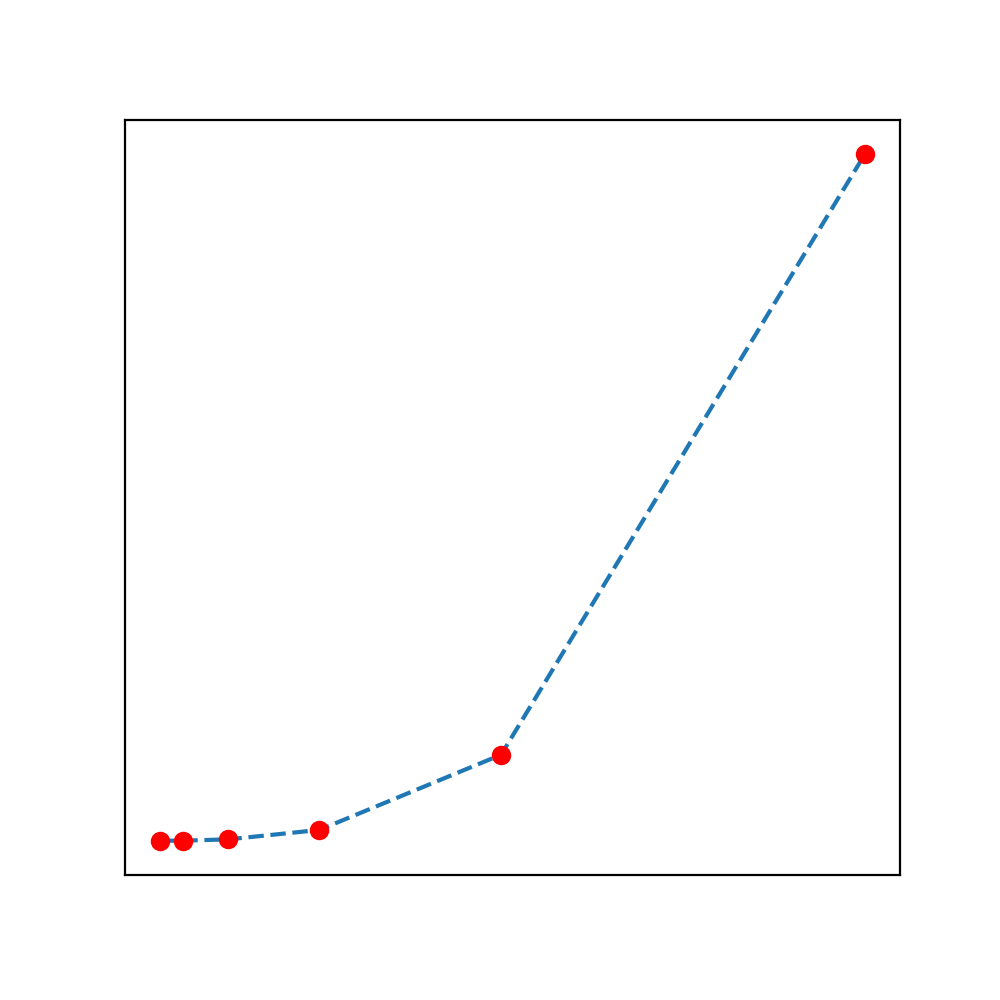
Fig: \(T(N)\) vs. \(N\)

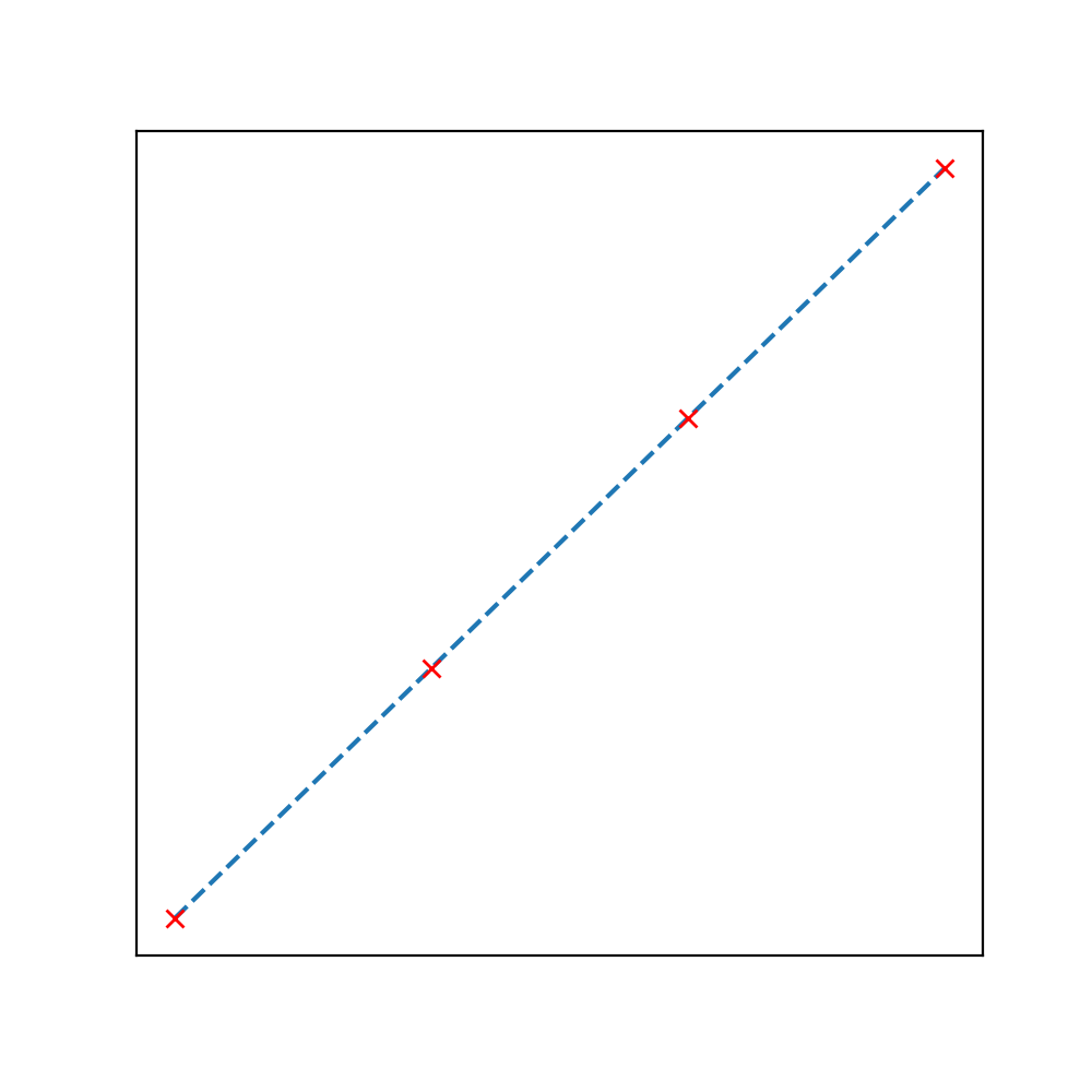
Fig: \(\log_2T(N)\) vs. \(\log_2 N\)

By using the data analysis approach, we should first plot \(T(n)\) against \(N\) and try to analyze the plot, in this step we can estimate if the relationship is linear (or not). But usually we are benefited more by plotting the same parameters on the log-log scale (base 2). If we do so, we are very likely to obtain a straight line and the slope of this line, \(b\) can be used in the power law relationship:

\[T(n) = aN^b \tag{1}\label{first}\]

where, \(a\) is a constant that can be determined by substituting the rest of the parameters (more on this later).

Note: In many cases, we may not be able to find a line that passes through each of the data points in our observation table and in that case, you can use linear regression to find an approximate one.

The equation of the obtained straight line on the log-log scale is:

\[\log_2(T(N)) = b\log_2 N + c\]

As evident, the slope of this line is \(b\) and the x-intercept is \(c\). Using both sides of this equation as exponents of 2, we get \(T(N) = aN^b\) where \(a = 2^c\).

Using linear regression (code provided later) we found the slope of the line to be 2.999 and by substituting this value in the power law equation (see eqn. \(\ref{first}\) ) (along with a set of observation from the table), we get the value of c to be -33.2103 and therefore, \(a = 1.006 \times 10^{-10}\). We arrive at a hypothesis that the running time of our algorithm can be determined for any input size \(N\) as \(1.006 \times 10^{-10} \times N^{2.999}\) seconds.

Now we can test our hypothesis by running the algorithm at different input sizes and then comparing the results with our predictions.

code example: using linear regression to fit observations to a straight line and then predicting.

import numpy as np
from sklearn.linear_model import LinearRegression

# some values have been omitted to avoid divide by zero error
x_vals = [1000, 2000, 4000, 8000]
y_vals = [0.1, 0.8, 6.4, 51.1]

# convert to numpy array and apply log function
x_vals = np.log2(np.array(x_vals).reshape(-1, 1))
y_vals = np.log2(np.array(y_vals).reshape(-1, 1))

# regress!
regressor = LinearRegression()
regressor.fit(x_vals, y_vals)

# slope of the line 
regressor.coef_
# > 2.999

# get predictions for input size of 16000
pred_log = regressor.predict(np.log2(np.array([16000]).reshape(-1, 1)))
pred = 2 ** pred_log
# > 408.8

doubling hypothesis

If there exists a power law relationship between \(T(n)\) and \(N\) for our algorithm, then we can use the doubling hypothesis as a quick way to estimate \(b\) in power law equation.

We need to prepare a table as shown below where the first two columns are the same as the previous table but the third column contains the ratio of the \(T(n_1)/T(n_2)\) where \(n_1 = 2n_2\) (also note that each value of \(n\) in the table is \(2 \times\)the previous value). The fourth column is \(log_2(\) value of ratio in the previous column \()\) i.e. \(log_2(T(2n)/T(n))\).

\[\begin{array} {|r|r|}\hline N & time (seconds) & ratio & lg\ ratio \\ \hline 250 & 0.0 & - & - \\ \hline 500 & 0.0 & 4.8 & 2.3 \\ \hline 1000 & 0.1 & 6.9 & 2.8 \\ \hline 2000 & 0.8 & 7.7 & 2.9 \\ \hline 4000 & 6.4 & 8.0 & 3.0 \\ \hline 8000 & 51.1 & 8.0 & 3.0 \\ \hline \end{array}\]

From the values in the table, it is evident that the value of ratio and the log of the ratio converge at a point (8.0 and 3.0 resp.) and the converged value of log of the ratio is the value of \(b\).

Explanation: The converged value of the ratio (third column) can be represented as:

\[ratio = \frac{a(2N)^b}{a(N)^b} = 2^b\]

and therefore, for the fourth column, we have:

\[log_2(ratio) = log_2(2^b) = b\]

note: it is not possible to identify logarithmnic factors using this method

In doubling hypothesis, we can estimate the value of \(a\) by substituting \(b\) in power law relationship for a large value of \(N\) and then solve for \(a\).

Considering \(N=8000, T(N) = 51.1\) and using the value of \(b=3\), we obtain:

\[\begin{align} 51.1 &= a \times 8000^3 \\ \implies a &= 0.998 \times 10^{-10} \end{align}\]

notes

In experimental algorithmics, the parameter \(b\) is system independent and is determined by the algorithm and the input data, while the parameter \(a\) is system dependent and is affected by the:

hardware: CPU, memory, cache, etc.
software: compiler, interpreter, garbage collector, etc.
system: OS, network, other running programs, etc.

references

Algorithms, Part 1 - Princeton University | Coursera - link

~ end of post ~